Testing Julia for Analysis of Neural Signals

This page explores possibilities of the new language Julia [julialang.org] for neural signal analyses. Hope is that it provides faster, user-friendly, web-centric alternative to the conventional Matlab programing.

Benchmark test

Comparison of Julia and Matlab by just a simple for-loop.
Julia

tic(); for i=1:1e8; 1+1; end; toc()
elapsed time: 0.22376203536987305 seconds

Matlab

tic; for i=1:1e8, 1+1; end; toc;
Elapsed time is 3.191013 seconds.

Thus, the Julia is very much promising!

The authors of the Julia say the reason why the Julia is fast and simple is its type system and multiple-dispatch. The input-output variables carry type information like C/Java, which makes the code fast. Like Matlab, however, you do not need to declare the types always. With the multiple-dispatch, functions with different types of input arguments can be defined using the same name. Combination of the two features makes the code fast and simple. However, this means we need to pay a little attention to types of the variables when they are used. For example, different operations + are called for 1+1 and 1+1.0, and they can behave differently if you define as such.

Density Estimation

Estimation of a probability density function from sampled data is often fundamental in statistical analysis. There are parametric and non-parametric approaches. Here we consider non-parametric methods. The most popular non-parametric methods are a histogram and kernel density estimation method. Here we consider the kernel density estimation and its optimization.

Data generation. Generate exponentially distributed data.

# Data
data = -log(rand(300,1))

Using function definition of Julia lang

# Gauss function
gauss(x,w) = 1/sqrt(2.0*pi)./w.*exp(-x.^2/2.0./w.^2)

the kernel density estimator is defined as

mean(gauss(x - data,w))

where x is the point of estimation. To obtain the Gauss function, a built-in gamma function may be used.

Use of comprehensions is powerful to create an array of function returns.

[mean(gauss(x - data,w)) | x = linspace(-1.0,3.0,100), w = .1]

Summary

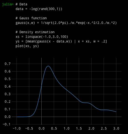
# Data
data = -log(rand(300,1))

# Gauss function
gauss(x,w) = 1/sqrt(2.0*pi)./w.*exp(-x.^2/2.0./w.^2) 

# Density estimation
xs = linspace(-1.0,3.0,100)
ys = [mean(gauss(x - data,w)) | x = xs, w = .2]
plot(xs, ys)

Bandwidth optimization

The kernel density estimation depends on the choice of bandwidth. It is possible to select an optimal bandwidth according to the data. The optimal bandwidth is given by the one that minimizes the following formula *

sskernel

where k_w is a kernel function with a bandwidth w. Here we consider the gauss kernel. This formula can be further simplified for a symmetric kernel. In addition, an explicit compacted formula is available for the gauss kernel function (see ref *). Here for simplicity and generality we compute the above formula.

To compute the above formula, we consider the sum of the gauss kernel function over the data points

[sum([sum(gauss(x - data, w)) | x = data]) | w=0.1]

if a bandwidth is 0.1.

Using the above expression, the formula is written as

c(w) = sum([sum(gauss(x-data,sqrt(2)*w))-2.0*sum(gauss(x-data,w))+2.0*gauss(0,w)| x = data])

We compute the cost functions for different bandwidths. Here the

# Bandwidths searched
ws = linspace(.01,0.5,50)

# Cost function
cs = [c(w) | w=ws]

We want to obtain w that minimizes this formula. Currently, the Julia's min function does not return the index of the minimum element. There are different ways. Here the we use the "ternary operator" ? to obtain the optimal bandwidth. It is useful as a short if-clause.

cmin = c[1]
idx = 1

for i = 1: length(c)
	idx = c[i] < cmin ? i : idx
	cmin = c[i] < cmin ? c[i] : cmin
end

wopt = ws[idx]

We will use wopt as the optimal bandwidth of kernel density estimation.

Summary of the Gauss kernel bandwidth optimization

# Data
data = -log(rand(400,1))

# Definition of Gauss kernel
gauss(x,w) = 1/sqrt(2.0*pi)./w.*exp(-x.^2/2.0./w.^2) 

# Bandwidths searched
ws = linspace(.01,0.5,50)

# Cost function
c(w) = sum([sum(gauss(x-data,sqrt(2)*w))-2.0*sum(gauss(x-data,w))+2.0*gauss(0,w)| x = data])
cs = [c(w) | w=ws]

# Plot the cost function
plot(ws,cs) 

# Select the optimal bandwidth
cmin = cs[1]
idx = 1
for i = 1: length(cs)
	idx = cs[i] < cmin ? i : idx
	cmin = cs[i] < cmin ? cs[i] : cmin
end
wopt = ws[idx]

# Plot the optimized density estimation
xs = linspace(-1.0,3.0,100)
ys = [mean(gauss(x - data,w)) | x = xs, w = wopt]
plot(xs, ys)

* Shimazaki H. and Shinomoto S., Kernel Bandwidth Optimization in Spike Rate Estimation
Journal of Computational Neuroscience (2010) Vol. 29 (1-2) 171-182 [Open Access: PDF, LINK]

Profile in Google+　